Evidence Synthesis: Meta-Analysis & Real-World Generalizability

Advanced Statistics for AI & Clinical Decision-Making — Lecture 4 of 4

Jonathan D. Stallings, PhD, MS

Data InDeed | dataindeed.org

2026-01-01

A rigorous estimate from one study is a starting point — not an answer. Evidence synthesis is how science accumulates.

What You’ll Learn Today

Post 09 — Meta-Analysis

• Why studies disagree and how to pool them
• Fixed-effects vs. random-effects models
• Forest plots and the I² statistic
• Bayesian meta-analysis and hierarchical pooling
• Heterogeneity as signal, not nuisance

Post 10 — RWE Generalizability

• Internal vs. external validity
• Generalizability vs. transportability
• Covariate reweighting for transport
• Site effects and multi-center data
• AI model performance transport

This is the capstone lecture of the Advanced Stats series. We’ve gone from data quality (missing data) through causal identification (propensity scores, IV, target trials) to now asking: even if our estimate is internally valid, does it apply beyond our study population? And if we have multiple studies — how do we combine them rigorously?

Part 1

Meta-Analysis

Combining evidence across studies

Why Studies Disagree: The Problem Meta-Analysis Solves

# Simulate 8 studies with true effect = -0.4, varying sample sizes and heterogeneity
studies <- tibble(
  study  = paste0("Study ", 1:8),
  n      = c(50, 120, 80, 200, 45, 300, 90, 150),
  effect = c(-0.6, -0.35, -0.55, -0.38, -0.22, -0.41, -0.70, -0.30),
  se     = sqrt(0.5 / n)
) |> mutate(
  lo = effect - 1.96*se,
  hi = effect + 1.96*se
)

ggplot(studies, aes(x=effect, y=reorder(study, effect))) +
  geom_point(aes(size=n), color="#0891b2") +
  geom_errorbarh(aes(xmin=lo, xmax=hi), height=0.25, color="#e2e8f0", linewidth=0.8) +
  geom_vline(xintercept=0, linetype=2, color="#e63946") +
  geom_vline(xintercept=-0.4, linetype=3, color="#22d3ee") +
  scale_size_continuous(range=c(2,7)) +
  labs(title="Eight studies — same question, different answers. Which do we believe?",
       x="Effect estimate (95% CI)", y=NULL, size="Sample n") + theme_di()

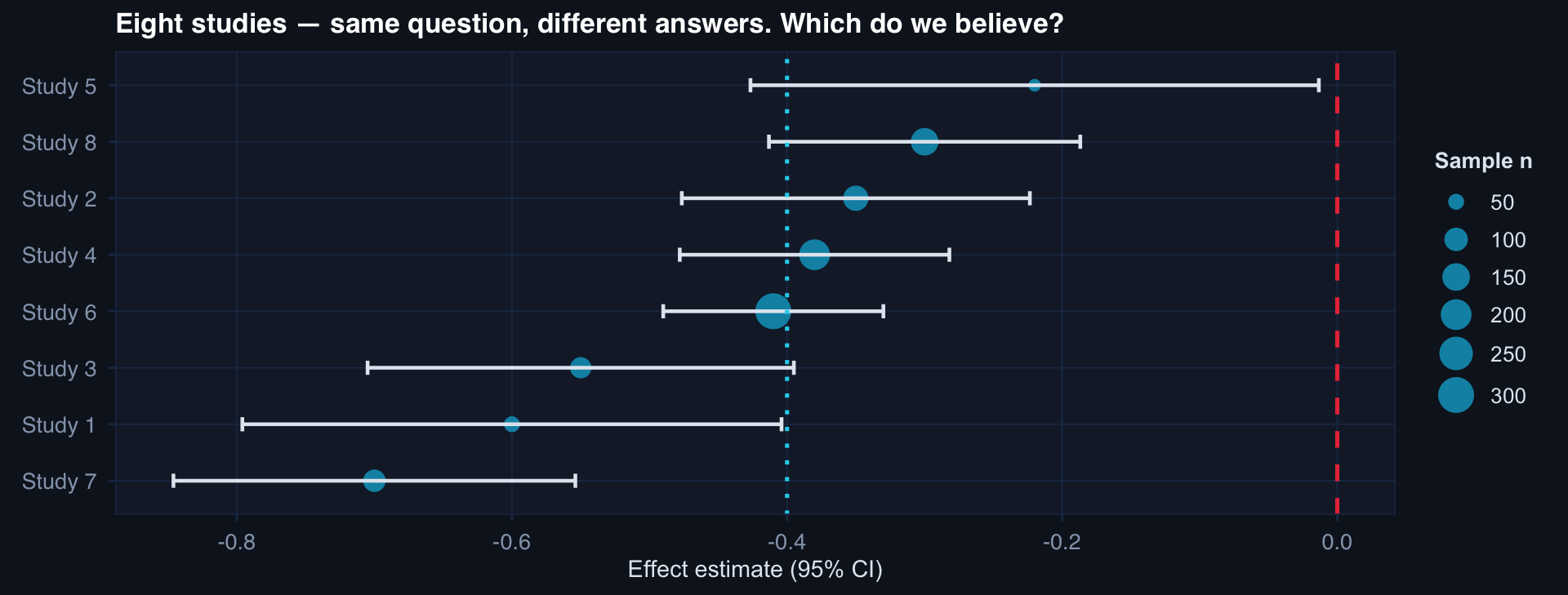
Point estimates range from −0.70 to −0.22. All are individually noisy. Meta-analysis pools them to a single, more precise estimate while quantifying between-study variability.

Fixed-Effects vs. Random-Effects Models

Fixed-effects: assumes one true common effect \(\mu\). Weights study \(k\) by \(w_k = 1/\sigma_k^2\).

\[\hat\mu_{FE} = \frac{\sum_k w_k \hat\theta_k}{\sum_k w_k}\]

Random-effects (DerSimonian-Laird): allows true effects to vary. \(\hat\theta_k \sim N(\mu, \tau^2)\).

\[\hat\mu_{RE} = \frac{\sum_k w_k^* \hat\theta_k}{\sum_k w_k^*}, \quad w_k^* = \frac{1}{\sigma_k^2 + \hat\tau^2}\]

	Fixed-effects	Random-effects
True effect	One universal value	Distribution of effects
Question answered	“What is the effect?”	“What is the average effect?”
Generalizability	Narrow (this population)	Broader (similar populations)
Sensitive to	Small high-precision studies	Between-study variance \(\tau^2\)

Computing the Pooled Estimate

# DerSimonian-Laird random-effects
theta <- studies$effect
se    <- studies$se
w_fe  <- 1 / se^2

# Fixed-effects pooled
mu_fe <- sum(w_fe * theta) / sum(w_fe)
se_fe <- sqrt(1 / sum(w_fe))

# Cochran's Q and tau^2
Q    <- sum(w_fe * (theta - mu_fe)^2)
df   <- nrow(studies) - 1
c_   <- sum(w_fe) - sum(w_fe^2)/sum(w_fe)
tau2 <- max(0, (Q - df) / c_)

# Random-effects pooled
w_re  <- 1 / (se^2 + tau2)
mu_re <- sum(w_re * theta) / sum(w_re)
se_re <- sqrt(1 / sum(w_re))

I2 <- max(0, (Q - df) / Q) * 100

tibble(
  Model     = c("Fixed-effects", "Random-effects"),
  Estimate  = round(c(mu_fe, mu_re), 3),
  SE        = round(c(se_fe, se_re), 3),
  `95% CI`  = paste0("[", round(c(mu_fe,mu_re)-1.96*c(se_fe,se_re),3),
                     ", ", round(c(mu_fe,mu_re)+1.96*c(se_fe,se_re),3), "]"),
  `tau^2`   = c(NA, round(tau2, 3)),
  `I^2 (%)`  = c(NA, round(I2, 1))
)

# A tibble: 2 × 6
  Model          Estimate    SE `95% CI`         `tau^2` `I^2 (%)`
  <chr>             <dbl> <dbl> <chr>              <dbl>     <dbl>
1 Fixed-effects    -0.418 0.022 [-0.461, -0.375]  NA          NA  
2 Random-effects   -0.435 0.048 [-0.529, -0.341]   0.013      76.5

The Forest Plot — Meta-Analysis Signature Visual

pooled <- tibble(
  study  = "Pooled (RE)",
  effect = mu_re, lo = mu_re - 1.96*se_re, hi = mu_re + 1.96*se_re,
  n = sum(studies$n)
)

bind_rows(studies, pooled) |>
  mutate(is_pooled = study=="Pooled (RE)",
         y_pos = row_number()) |>
  ggplot(aes(x=effect, y=reorder(study, y_pos),
             color=is_pooled, size=is_pooled)) +
  geom_point() +
  geom_errorbarh(aes(xmin=lo, xmax=hi), height=0.3, linewidth=0.7) +
  geom_vline(xintercept=0, linetype=2, color="#e63946", linewidth=0.8) +
  scale_color_manual(values=c("#0891b2","#f59e0b")) +
  scale_size_manual(values=c(2.5, 5)) +
  labs(title=paste0("Forest plot — I² = ", round(I2,1), "% (moderate heterogeneity)"),
       x="Effect estimate (95% CI)", y=NULL) +
  theme_di() + theme(legend.position="none")

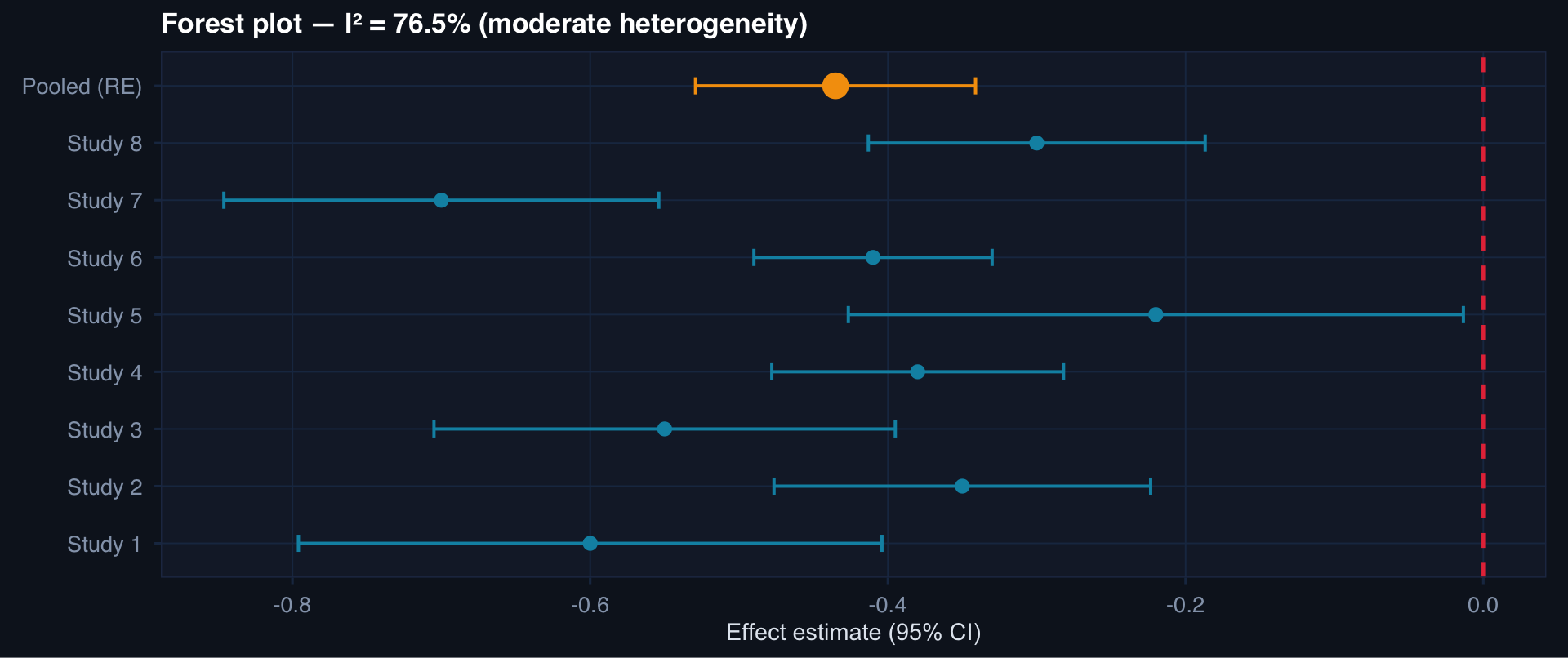
I² interpretation: < 25% = low heterogeneity. 25–75% = moderate — heterogeneity is real and worth investigating. > 75% = high — pooled estimate may be misleading; explore subgroups.

Heterogeneity Is Signal, Not Nuisance

When \(I^2\) is high, the right response is not to force a single pooled estimate — it’s to ask why studies differ.

Sources of heterogeneity to investigate:

• Patient population (civilian vs. military, age, mechanism)
• Treatment definition (timing, dose, protocol variation)
• Outcome definition (30-day vs. in-hospital mortality)
• Study quality and design
• Publication bias (funnel plot asymmetry)

DoDTR application: A meta-analysis of tourniquet efficacy across civilian and military trauma systems will show high \(I^2\) — not because the studies are wrong, but because the effect genuinely differs by context (pre-hospital time, injury mechanism, Role of care). That’s scientifically important information.

Part 2

Real-World Generalizability

Does your finding travel?

Internal vs. External Validity

Internal validity: Is the estimate causally valid within the study population?

→ Randomization, propensity scores, IV, target trial emulation address this.

External validity (generalizability): Does the estimate apply to a different population?

→ Requires that effect modifiers have the same distribution in the target population.

Generalizability vs. Transportability:

Generalizability: from a non-representative sample to the broader source population (e.g., from one trauma center to all Level I centers).

Transportability: from one population to a different target population (e.g., from US civilian trauma to NATO military trauma).

The second is harder — requires assumptions about effect-modifier distributions.

Covariate Shift: The Mechanism of External Validity Failure

# Source population (US civilian trauma) vs. target (military combat trauma)
n_src <- 400; n_tgt <- 300

df_ext <- bind_rows(
  tibble(pop="Source (civilian)", iss=rnorm(n_src, 22, 10),
         age=rnorm(n_src, 42, 18), penetrating=rbinom(n_src,1,0.20)),
  tibble(pop="Target (military)", iss=rnorm(n_tgt, 32, 12),
         age=rnorm(n_tgt, 26, 6),  penetrating=rbinom(n_tgt,1,0.65))
)

df_ext |>
  pivot_longer(c(iss, age)) |>
  ggplot(aes(value, fill=pop, color=pop)) +
  geom_density(alpha=0.4, linewidth=0.8) +
  facet_wrap(~name, scales="free",
             labeller=labeller(name=c(age="Age (years)", iss="ISS"))) +
  scale_fill_manual(values=c("#2563eb","#e63946")) +
  scale_color_manual(values=c("#2563eb","#e63946")) +
  labs(title="Source vs. target population: ISS and age distributions are very different",
       fill=NULL, color=NULL) + theme_di()

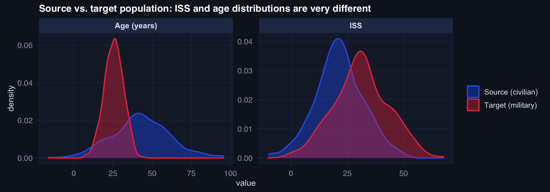
A mortality model trained on civilian trauma patients (older, blunt mechanism, lower ISS) will systematically misfires on military combat casualties (younger, penetrating, higher ISS).

Transportability Reweighting

n <- 500
# Source data with outcome
df_src <- tibble(
  iss  = rnorm(n, 22, 10),
  age  = rnorm(n, 42, 18),
  pop  = 0L,
  outcome = 5 + 0.15*iss - 0.02*age + rnorm(n, 0, 3)
)
# Target data (no outcome)
df_tgt <- tibble(
  iss  = rnorm(300, 32, 12),
  age  = rnorm(300, 26, 6),
  pop  = 1L,
  outcome = NA_real_
)

# Estimate inverse odds weights for transportability
df_combined <- bind_rows(df_src, df_tgt)
pop_model   <- glm(pop ~ iss + age, data=df_combined, family=binomial)
df_src$iow  <- predict(pop_model, newdata=df_src, type="response") /
               (1 - predict(pop_model, newdata=df_src, type="response"))

# Unadjusted source effect vs. transported estimate
src_mean    <- mean(df_src$outcome)
transp_mean <- weighted.mean(df_src$outcome, df_src$iow)

cat("Source mean outcome:       ", round(src_mean, 3))

Source mean outcome:        7.597

cat("\nTransported to target mean:", round(transp_mean, 3))

Transported to target mean: 9.39

cat("\n\nTrue target mean (oracle): ~", round(5 + 0.15*32 - 0.02*26, 2))

True target mean (oracle): ~ 9.28

AI Model Performance Transport

The same problem applies to predictive models, not just causal estimates:

# Train mortality model on source, evaluate on source vs. target
set.seed(42)
df_train <- tibble(
  iss  = rnorm(400, 22, 10),
  sbp  = rnorm(400, 112, 22),
  died = rbinom(400, 1, plogis(-3 + 0.08*iss - 0.01*sbp))
)
df_target <- tibble(
  iss  = rnorm(200, 32, 12),
  sbp  = rnorm(200, 100, 28),
  died = rbinom(200, 1, plogis(-3 + 0.08*iss - 0.01*sbp))
)

fit <- glm(died ~ iss + sbp, data=df_train, family=binomial)

pred_src <- predict(fit, type="response")
pred_tgt <- predict(fit, newdata=df_target, type="response")

tibble(
  Population   = c("Source (train/validate)", "Target (military)"),
  `Mean pred.` = round(c(mean(pred_src), mean(pred_tgt)), 3),
  `Obs. rate`  = round(c(mean(df_train$died), mean(df_target$died)), 3),
  Calibration  = c("✓ Expected", "⚠ Check required")
)

# A tibble: 2 × 4
  Population              `Mean pred.` `Obs. rate` Calibration     
  <chr>                          <dbl>       <dbl> <chr>           
1 Source (train/validate)        0.128       0.128 ✓ Expected      
2 Target (military)              0.246       0.245 ⚠ Check required

The deployment gap: A TRISS-based mortality model trained on US civilian registry data will be miscalibrated when deployed on combat casualty data — different ISS distribution, different age profile, different mechanism mix. Recalibration or reweighting is required before deployment.

Advanced Statistics Series — Complete

Lecture 1: Missing Data

• MCAR/MAR/MNAR — mechanism matters
• MICE for inference; sensitivity for MNAR
• Tipping-point analysis for communication

Lecture 2: Causal Inference

• Potential outcomes + estimand clarity
• Propensity scores: balance ≠ model fit
• Love plots, SMD, IPTW

Lecture 3: Identification

• IV for unmeasured confounding
• DAGs before models
• Target trial emulation as design discipline

Lecture 4: Evidence Synthesis

• Fixed vs. random effects meta-analysis
• I² is a signal to investigate, not suppress
• Transportability ≠ generalizability
• Reweight for the target — don’t assume portability

The series thesis: Observational data can produce rigorous evidence — but only when analysts reason carefully about why data are missing, how treatment was assigned, what question is being asked, and whether the answer travels.

Full Advanced Statistics Reading List

Missing Data:

• Decoding Missing Data: MCAR/MAR/MNAR
• Filling the Gaps: Imputation Strategies
• What If? Sensitivity Analysis

Causal Inference:

• From Correlation to Causation
• Propensity Scores: Balancing the Scales

Identification:

• Instrumental Variables
• Taming Confounders
• Emulating Trials with Real Data

Synthesis:

• Meta-Analysis Mastery
• Beyond the Lab: Making RWE Generalizable