Mathematical Foundations of Modern AI

Applied Statistics for AI & Clinical Decision-Making — Lecture 10 of 10

Jonathan D. Stallings, PhD, MS

Data InDeed | dataindeed.org

2026-01-01

Every model we’ve covered runs on these three engines: optimization, linear algebra, and calculus.

What You’ll Learn Today — And Why Now

Post 24 Optimization

• Gradient descent
• Learning rate
• Stochastic & mini-batch

Post 25 Linear Algebra

• Vectors & matrices
• Eigendecomposition
• SVD

Post 26 Calculus

• Derivatives & gradients
• Chain rule
• Automatic differentiation

We cover these last because you’ve now seen them in action. Optimization powered your logistic regression. Linear algebra powered PCA. Calculus powered every gradient you’ve implicitly computed.

Part 1

Optimization

The engine that trains every model

What We’re Optimizing

Every model training is an optimization problem:

\[\hat{\theta} = \arg\min_\theta \mathcal{L}(\theta; \text{data})\]

Model	Loss function \(\mathcal{L}\)
Linear regression	Mean squared error
Logistic regression	Binary cross-entropy
Lasso	RSS + λ|β|₁
Neural network	Cross-entropy or MSE
Cox model	Negative partial log-likelihood

Gradient descent is the universal algorithm for finding the minimum when an analytic solution doesn’t exist.

Gradient Descent: Step Downhill

\[\theta_{t+1} = \theta_t - \alpha \nabla_\theta \mathcal{L}(\theta_t)\]

\(\alpha\) = learning rate (step size)

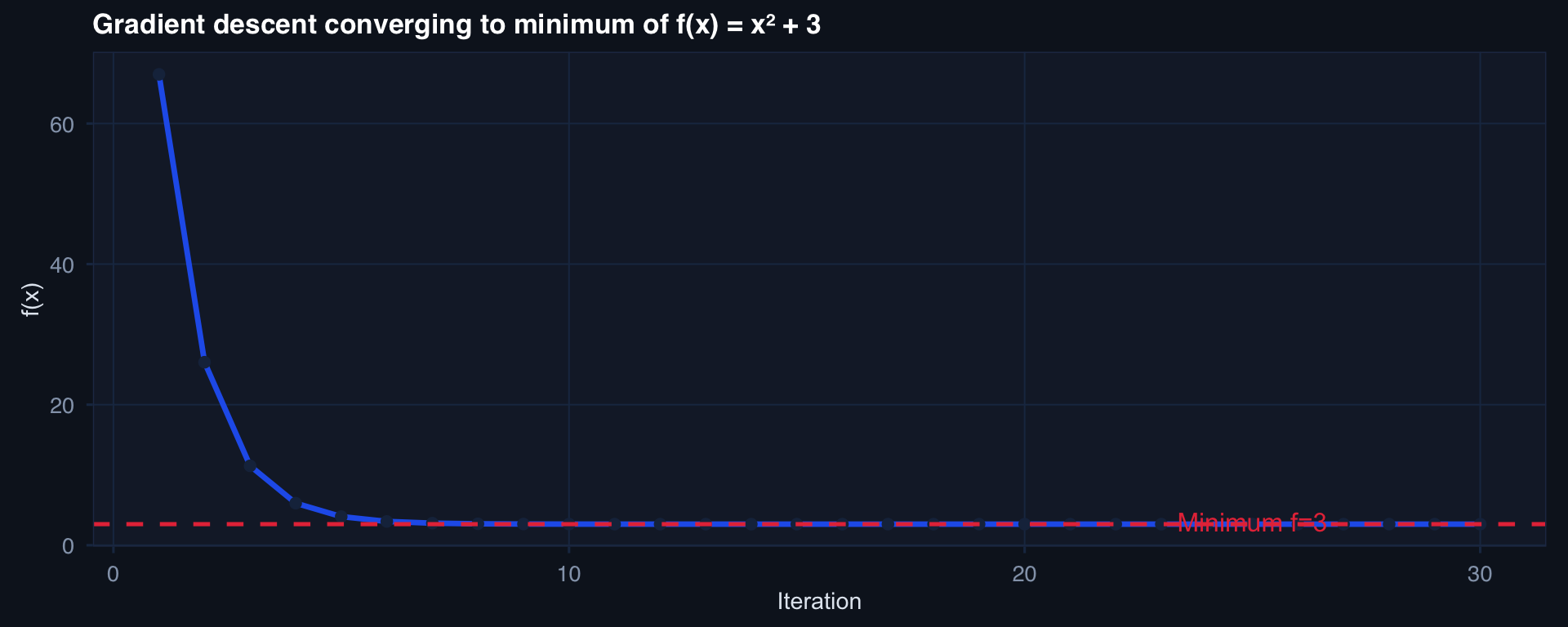
# Simple example: minimize f(x) = x^2 + 3
x_path <- numeric(30); x_path[1] <- 8; lr <- 0.2
for(i in 2:30) x_path[i] <- x_path[i-1] - lr * 2 * x_path[i-1]

tibble(iter=1:30, x=x_path, f=x_path^2+3) |>
  ggplot(aes(iter, f)) +
  geom_line(linewidth=1.2, color="#2563eb") +
  geom_point(size=2, color="#1b2e4b") +
  geom_hline(yintercept=3, linetype=2, color="#e63946") +
  annotate("text",x=25,y=3.3,label="Minimum f=3",color="#e63946") +
  labs(title="Gradient descent converging to minimum of f(x) = x² + 3",
       x="Iteration", y="f(x)") + theme_di()

Gradient descent is the algorithm that makes deep learning possible. Every time you train a logistic regression with glm(), R is internally solving the normal equations or running a Newton-Raphson iteration — which is second-order gradient descent. For neural networks with millions of parameters, first-order gradient descent (often mini-batch SGD or Adam) is the only tractable option.

Learning Rate: The Most Important Hyperparameter

run_gd <- function(lr, n_iter=40) {
  x <- 8
  sapply(1:n_iter, function(i) { x <<- x - lr * 2 * x; x^2 + 3 })
}
tibble(iter=rep(1:40,3),
       loss=c(run_gd(0.05), run_gd(0.2), run_gd(0.6)),
       lr=rep(c("Too small (0.05)","Just right (0.2)","Too large (0.6)"), each=40)) |>
  ggplot(aes(iter, loss, color=lr)) +
  geom_line(linewidth=1) +
  scale_y_log10() +
  scale_color_manual(values=c("#94a3b8","#2563eb","#e63946")) +
  labs(title="Learning rate: too small = slow, too large = diverges",
       x="Iteration", y="Loss (log scale)", color=NULL) + theme_di()

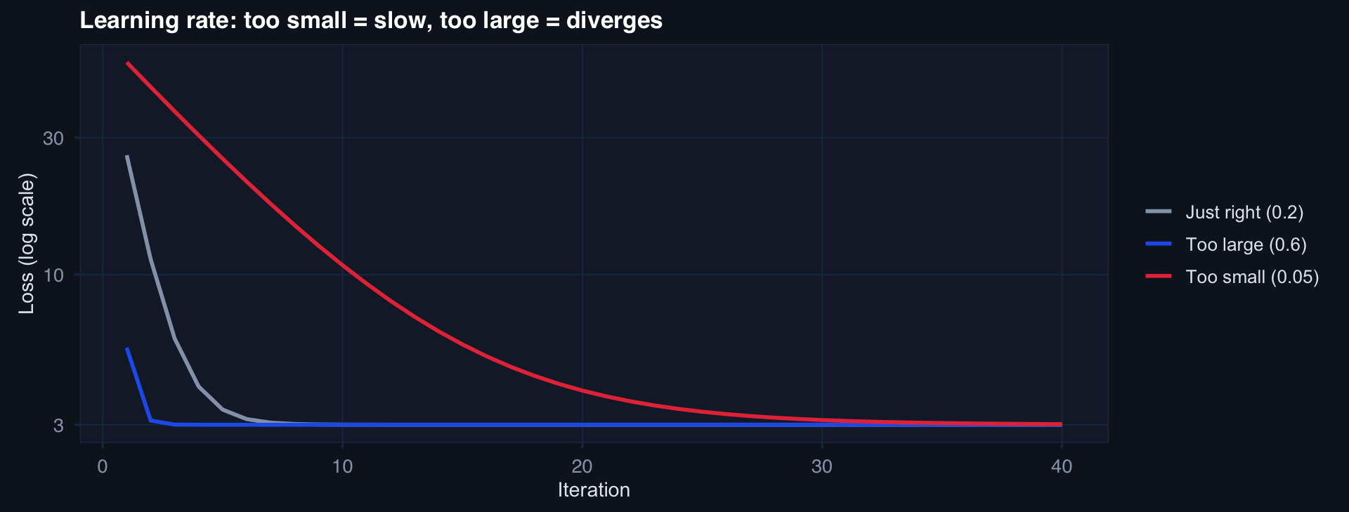
Too small → converges very slowly. Too large → overshoots minimum, diverges. Just right → fast, stable convergence.

Part 2

Linear Algebra

The data structure underneath every computation

Why Linear Algebra Is Everywhere

Every dataset is a matrix. Every prediction is a matrix operation.

Linear regression: \(\hat{y} = X\hat{\beta} = X(X^\top X)^{-1}X^\top y\)

PCA: \(X = U D V^\top\) (SVD)

Neural forward pass: \(a^{(l)} = \sigma(W^{(l)} a^{(l-1)} + b^{(l)})\)

X <- matrix(c(1,2,3,4,5,6), nrow=3, byrow=TRUE)
cat("X:\n"); print(X)

X:

     [,1] [,2]
[1,]    1    2
[2,]    3    4
[3,]    5    6

cat("\nX'X:\n"); print(t(X) %*% X)

X'X:

     [,1] [,2]
[1,]   35   44
[2,]   44   56

cat("\nSingular values:", round(svd(X)$d, 3))

Singular values: 9.526 0.514

SVD: The Most Important Matrix Decomposition

\[X = U D V^\top\]

• \(U\): left singular vectors (row space)
• \(D\): singular values (importance of each direction)
• \(V\): right singular vectors (column space)

# Simulate patient × feature matrix, reconstruct with k=2 components
n <- 100; p <- 8
X_patients <- scale(matrix(rnorm(n*p), n, p))
svd_fit <- svd(X_patients)

# Low-rank approximation with k=2
k <- 2
X_approx <- svd_fit$u[,1:k] %*% diag(svd_fit$d[1:k]) %*% t(svd_fit$v[,1:k])
cat("Variance explained by 2 components:",
    round(sum(svd_fit$d[1:2]^2) / sum(svd_fit$d^2), 3))

Variance explained by 2 components: 0.36

PCA is SVD on the centered data matrix. Understanding SVD means understanding PCA, matrix completion, recommendation systems, and latent semantic analysis.

Part 3

Calculus

Derivatives as the language of change

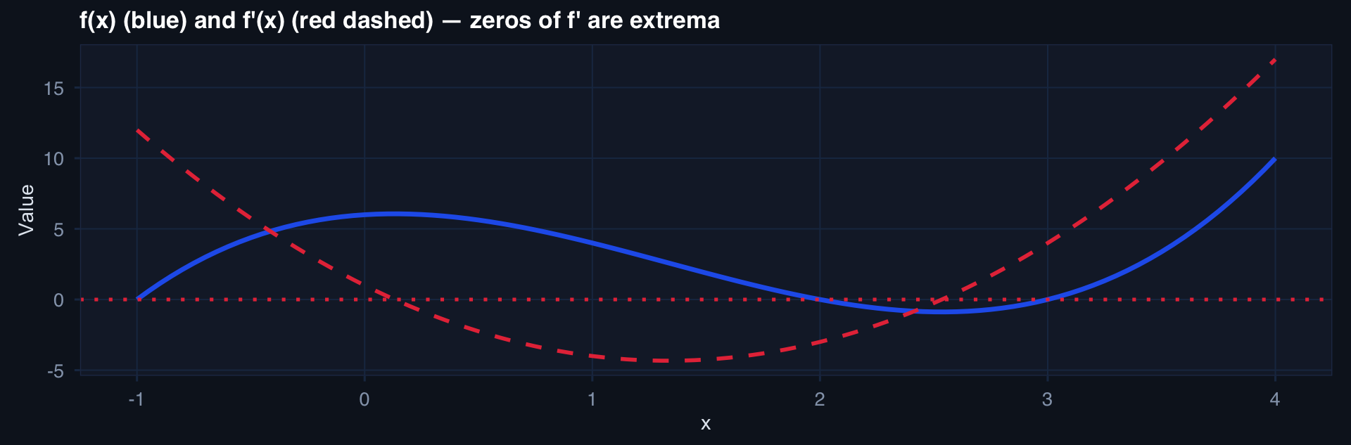
The Derivative: Rate of Change

\[f'(x) = \lim_{h \to 0} \frac{f(x+h) - f(x)}{h}\]

For a multivariable function: gradient \(\nabla_\theta \mathcal{L} = \left[\frac{\partial \mathcal{L}}{\partial \theta_1}, \dots, \frac{\partial \mathcal{L}}{\partial \theta_k}\right]^\top\)

f   <- function(x) x^3 - 4*x^2 + x + 6
df  <- function(x) 3*x^2 - 8*x + 1

x_grid <- seq(-1, 4, 0.05)
tibble(x=x_grid, f=f(x_grid), deriv=df(x_grid)) |>
  ggplot(aes(x)) +
  geom_line(aes(y=f), color="#2563eb", linewidth=1.2) +
  geom_line(aes(y=deriv), color="#e63946", linewidth=1, linetype=2) +
  geom_hline(yintercept=0, linetype=3) +
  labs(title="f(x) (blue) and f'(x) (red dashed) — zeros of f' are extrema",
       y="Value") + theme_di()

The Chain Rule: How Backprop Works

\[\frac{d}{dx}[f(g(x))] = f'(g(x)) \cdot g'(x)\]

In neural networks: backpropagation applies the chain rule layer by layer, from loss back to first-layer weights.

# Automatic differentiation concept — numerical illustration
# dL/dw = dL/da × da/dz × dz/dw
dL_da  <- -2.5    # gradient from loss
da_dz  <- 0.18    # sigmoid derivative at activation z
dz_dw  <- 1.3     # input value = dz/dw for linear layer

dL_dw  <- dL_da * da_dz * dz_dw
cat("Chain rule: dL/dw =", dL_da, "×", da_dz, "×", dz_dw, "=", round(dL_dw,4))

Chain rule: dL/dw = -2.5 × 0.18 × 1.3 = -0.585

This same product of derivatives, applied at every weight in a deep network, is backpropagation. The chain rule is why neural networks are trainable.

Lecture 10 — Key Takeaways

Optimization

• GD: θ ← θ − α∇L
• Learning rate controls speed and stability
• SGD/mini-batch GD for large datasets
• Adam optimizer adapts learning rate per parameter

Linear Algebra

• Data = matrix; prediction = matrix multiplication
• SVD underlies PCA, compression, latent representation
• Eigenvalues tell you dominant variance directions
• Matrix inversion is numerically fragile — prefer factorizations

Calculus

• Derivative = instantaneous rate of change
• Gradient = direction of steepest ascent in multivariable space
• Chain rule → backpropagation → neural network training
• Automatic differentiation (PyTorch, JAX, Stan) does this for you

The meta-lesson: You can use every model in this course without deriving these from scratch. But knowing the machinery makes you a better analyst — you understand what can go wrong and why.

Series Complete — What You Can Do Now

10 lectures · 30 posts · ~8.5 hours

Foundation (Lectures 1–3)

• Reason probabilistically under uncertainty
• Estimate parameters and communicate uncertainty honestly
• Avoid the p-value traps that corrupt most clinical research

Modeling (Lectures 4–6)

• Build Bayesian models with priors from clinical knowledge
• Fit regression models appropriate to the outcome type
• Analyze time-to-event data correctly with censoring

Modern ML (Lectures 7–9)

• Navigate high-dimensional data without overfitting
• Evaluate models honestly — discrimination AND calibration
• Build ensembles that outperform single models

Foundations (Lecture 10)

• Understand what gradient descent is actually doing
• Read linear algebra in model outputs (PCA, SVD)
• Trace a backpropagation derivative by hand

Coming next: Advanced Statistics Series → Experimental Design Series

The Applied Statistics Series — Full Reading List

Lectures 1–5: 1. How Probability Powers Everyday AI 2. Demystifying Random Variables 3. Top Probability Distributions 4. The CLT Magic 5. LLN in Action 6–13. (Lectures 2–4 posts) 14. ANOVA in ML 15. PCA Demystified

Lectures 6–10: 16–22. (Lectures 6–8 posts) 23. Entropy in Stats 24. Optimization Essentials 25. Linear Algebra for Stats Pros 26. Calculus Crash Course 27. Monte Carlo Magic 28. Beating the Curse of Dimensionality 29. Metrics That Matter 30. Ensembles